因为不想自己配环境,所以就直接用现成机器学习平台。
这里用的是 Google 下面的 Colab (如果没有小飞机的话可以用阿里云的机器学习 PAI,这是一个很新的平台)
完整文件在 github 上:机器学习作业1
(帮忙点个小星星呗,孩子不容易啊😂)
线性回归
某城市的电网系统需要升级,以应对日益增长的用电需求。电网系统需要考虑最高温度对城市的峰值用电量的影响。项目负责人需要预测明天城市的峰值用电量,他搜集了以往的数据。现在,负责人提供了他搜集到的数据,并请求你帮他训练出一个模型,这个模型能够很好地预测明天城市的峰值用电量。
1- 准备
先导入必要的python包
In [107]:
import numpy as np
import matplotlib.pyplot as plt
import time
%matplotlib inline
导入负责人提供的数据,并可视化数据
In [113]:
data = np.loadtxt('/content/drive/MyDrive/data.txt')
#data 第一列为温度信息 第二列为人口信息
X = data[:,0].reshape(-1,1)
#data 第三列为用电量信息
Y = data[:,2].reshape(-1,1)
plt.xlabel('High temperature')
plt.ylabel('Peak demand ')
plt.scatter(X,Y)
print('X shape:',X.shape)
print('Y shape:',Y.shape)
print('some X[:5]:',X[:5])
print('some Y[:5]:',Y[:5])
X shape: (80, 1)
Y shape: (80, 1)
some X[:5]: [[37.24]
 [37.53]
 [33.92]
 [26.59]
 [20.05]]
some Y[:5]: [[4.04]
 [2.84]
 [3.2 ]
 [3.42]
 [2.32]]

In [12]:
from google.colab import drive
drive.mount('/content/drive')
Mounted at /content/drive
2- 单变量线性回归
你决定使用回归算法来训练一个模型,用来预测明天城市的峰值用电量。
单变量线性回归模型表示

单变量线性回归的模型由两个参数,
来表示一条直线。我们的目标也就是找到一个”最符合”的直线或者说参数
如何选择。
设输入的特征——最高温度(F)为,
。
为样本总数,在该例子中为
。
为特征的个数,这里为
。
设输出为,表示第
天的峰值用电量。
参数为
在该例子中,模型应该为一条直线,假设模型为:注意:这里的
是一个向量,
是标量。使用向量化的表示原因(1)简化数学公式的书写(2)与程序代码中的表示可以一致,使用向量化的代码表示可以加速运算,因此一般能不用
for循环的地方都不用for循环。
下面一个简单的例子说明向量化的代码运算更快
In [78]:
# 随机初始化两个向量,计算它们的点积
x = np.random.rand(10000000,1)
y = np.random.rand(10000000,1)
ans = 0
start = time.time()
for i in range(10000000):
    ans += x[i,0]*y[i,0]
end = time.time()
print('for循环的计算时间%.2fs'%(end - start))
print('计算结果:%.2f'%(ans))
start = time.time()
ans = np.dot(x.T,y)
end = time.time()
print('向量化的计算时间%.2fs'%(end - start))
print('计算结果:%.2f'%(ans))
for循环的计算时间8.03s
计算结果:2498917.85
向量化的计算时间0.01s
计算结果:2498917.85
因为 因此,为了方便编程,我们需要给每一个
的前面再加一行1。使得每一个
成为了一个2维向量
预测结果
模型需要根据输入自变量 和参数
来预测可能的产生的
直接将自变量 作为模型的输入,而模型自动根据输入和当前参数
输出预测结果:
其中 为模型在参数为
情况下,对于输入
的预测函数。
为当前情况下模型根据输入而做出的预测
在预测阶段, 作为自变量
损失函数
模型的预测结果和实际结果有差距,为了衡量它们之间的差距,或者说使用这个模型产生的损失,我们定义损失函数
这里我们使用平方损失:
上述损失函数表示一个样本的损失,整个训练集的损失使用表示:
(其中数字2的作用是方便求导时的运算)
为了使模型的预测效果好,需要最小化训练集上的损失,。
在损失阶段, 作为自变量
梯度下降法
为了得到使得损失函数最小化的
,可以使用梯度下降法。
损失函数的函数图像如下

损失函数关于参数向量
中的一个参数比如
的函数图是
假设一开始的值在紫色点上,为了降低
值,需要
往右变移动,这个方向是
在
上的负梯度。只要
不断往负梯度方向移动,
一定可以降到最低值。梯度下降法就是使参数
不断往负梯度移动,经过有限次迭代(更新
值)之后,损失函数
达到最低值。
梯度下降法的过程:
- 初始化参数向量
。
-
开始迭代
A.根据实际输入
和参数
B. 根据预测输出值和实际输出值之间的差距,计算损失函数
,
C. 计算
D. 更新参数
现在,我们开始实现 Regression 学习算法。
任务1: 首先在前面加上一列1,表示参数
的系数,方便运算。
是形状为
的矩阵,一共
行数据,我们需要为每一行数据的前面加一列1,也就是像这样
提示:可以使用np.hstack把两个矩阵水平合在一起。用1初始化向量或矩阵的函数是np.ones。(函数详情使用python的帮助函数help,比如help(np.ones),或者百度。)
In [114]:
def preprocess_data(X):
    """输入预处理 在X前面加一列1
    参数:
        X:原始数据,shape为 mx1
    返回:
        X_train: 在X加一列1的数据,shape为 mx2
    """

    m = X.shape[0]   # m 是数据X的行数
    ### START CODE HERE ###

    X_train = np.hstack((np.array(np.ones(m))[:, np.newaxis],X))

    ### END CODE HERE ###
    return X_train
In [115]:
X = preprocess_data(X)
print('new X shape:',X.shape)
print('Y shape:',Y.shape)
print('new X[:10,:]=',X[:5,:])
print('Y[:10,:]=',Y[:5,:])
new X shape: (80, 2)
Y shape: (80, 1)
new X[:10,:]= [[ 1.   37.24]
 [ 1.   37.53]
 [ 1.   33.92]
 [ 1.   26.59]
 [ 1.   20.05]]
Y[:10,:]= [[4.04]
 [2.84]
 [3.2 ]
 [3.42]
 [2.32]]
任务2: 接着,初始化参数向量。
的shape是
,我们随机初始化
。
提示:numpy的随机函数是np.random.rand。
In [116]:
def init_parameter(shape):
    """初始化参数
    参数:
        shape: 参数形状
    返回:
        theta_init: 初始化后的参数

    """
    np.random.seed(0)
    m, n = shape
    ### START CODE HERE ###
    theta_init = np.random.rand(m,n)

    ### END CODE HERE ###

    return theta_init
In [117]:
theta = init_parameter((2,1))
print('theta shape is ',theta.shape)
print('theta = ',theta)
theta shape is  (2, 1)
theta =  [[0.5488135 ]
 [0.71518937]]
任务3:通过已知 和参数
计算预测的
值。由于使用
for循环单独计算每个预测值效率不高,因此我们需要用向量化的方法去掉for循环。
大小为
(
表示特征数量,对于这里
),每行是一条样本特征向量,
大小为
,可以使用
计算所有样本的预测结果,大小为
这里的线性模型就可以表示为, 这里
的大小为
,结果上等于
提示:矩阵相乘 np.dot(矩阵1,矩阵2)
In [118]:
def compute_predict_Y(X,theta):
    ### START CODE HERE ###
    predictY = np.dot(X,theta)
    ### END CODE HERE ###
    return predictY
predict_Y = compute_predict_Y(X,theta)
print(predict_Y[:5])
[[27.18246551]
 [27.38987042]
 [24.80803681]
 [19.56569876]
 [14.8883603 ]]
任务4: 实现计算损失函数的函数。
从公式
我们可以看到有个求和。由于使用for循环效率不高,因此我们需要用向量化的方法去掉for循环。接着
计算所有样本的损失值,最后求和并除以得到
的值。因此,,
应该是一个标量
提示:矩阵乘法运算可使用np.dot函数,平方运算可使用np.power(data, 2)函数,求和运算可使用np.sum。
In [119]:
def compute_J(predict_Y, Y):
    """计算损失函数J
    参数:
        X: 训练集数据特征,shape: (m, 2)
        Y: 训练集数据标签,shape: (m, 1)
        theta: 参数,shape: (2, 1)

    返回:
        loss: 损失值
    """

    m = Y.shape[0]

    ### START CODE HERE ###


    loss = np.sum(np.power(np.subtract(predict_Y,Y),2))/(2*m)

    ### END CODE HERE ###

    return  loss
In [120]:
first_loss = compute_J(predict_Y, Y)
print("first_loss = ", first_loss)
first_loss = 144.24776230557214
任务5:计算参数的梯度。
向量化公式为
提示:矩阵A的转置表示为A.T
In [121]:
def compute_gradient(predict_Y, Y):
    """计算参数theta的梯度值
    参数:
        X: 训练集数据特征,shape: (m, 2)
        Y: 训练集数据标签,shape: (m, 1)
        theta: 参数,shape: (2, 1)

    返回:
        gradients: theta的梯度列表 shape:(2,1)
    """

    m = X.shape[0]
    gradients = None

    ### START CODE HERE ###

    gradients = np.dot(X.T,np.subtract(np.dot(X,theta),Y))
    gradients /= m

    ### END CODE HERE ###

    return gradients
In [122]:
gradients_first = compute_gradient(predict_Y, Y)
print("gradients_first shape : ", gradients_first.shape)
print("gradients_first = ", gradients_first)
gradients_first shape :  (2, 1)
gradients_first =  [[ 16.01688437]
 [460.53440708]]
任务6:用梯度下降法更新参数
提示:
parameters =
–
实现update_parameters函数。
In [123]:
def update_parameters(theta, gradients, learning_rate=0.01):
    """更新参数theta
    参数:
        theta: 参数,shape: (2, 1)
        gradients: 梯度,shape: (2, 1)
        learning_rate: 学习率,默认为0.01

    返回:
        parameters: 更新后的参数
    """
    ### START CODE HERE ###

    parameters = np.subtract(theta,learning_rate*gradients)
    ### END CODE HERE ###

    return parameters
In [124]:
theta_one_iter = update_parameters(theta, gradients_first, 0.01)

print("theta_one_iter = ", theta_one_iter)
theta_one_iter =  [[ 0.38864466]
 [-3.8901547 ]]
任务7:将前面定义的函数整合起来,实现完整的模型训练函数。迭代更新
iter_num次。迭代次数参数iter_num也是一个超参数,如果iter_num太小,损失函数还没有收敛;如果
iter_num太大,损失函数早就收敛了,过多的迭代浪费时间。
In [125]:
def model(X, Y, theta, iter_num = 100, learning_rate=0.0001):
    """梯度下降函数
    参数:
        X: 训练集数据特征,shape: (m, n+1)
        Y: 训练集数据标签,shape: (m, 1)
        iter_num: 梯度下降的迭代次数
        theta: 初始化的参数,shape: (n+1, 1)
    返回:
        loss_history: 每次迭代的损失值
        theta_history: 每次迭代更新后的参数
        theta: 训练得到的参数
    """

    loss_history = []
    theta_history = []

    for i in range(iter_num):

        ### START CODE HERE ###
        # 预测
        predict_Y = compute_predict_Y(X,theta)
        # 计算损失
        loss = compute_J(predict_Y, Y)
        # 计算梯度
        gradients = compute_gradient(predict_Y, Y)
        # 更新参数
        theta = update_parameters(theta, gradients, learning_rate)
        ### END CODE HERE ###

        loss_history.append(loss)
        theta_history.append(theta)

    return loss_history, theta_history, theta
In [126]:
# 尝试不同的学习率和迭代次数
# 提交作业之前要把学习效率改为0.0001,然后重新运行一遍

loss_history, theta_history, theta = model(X, Y, theta, 14, learning_rate=0.0001)

print("theta = ", theta)

plt.plot(loss_history)
print("loss = ", loss_history[-1])
theta =  [[0.52638987]
 [0.0704412 ]]
loss =  0.35305686809016384

下面是学习到的线性模型与原始数据的关系
In [48]:
plt.scatter(X[:,1],Y)
x = np.arange(10,42)
plt.plot(x,x*theta[1][0]+theta[0][0],'r')
Out[48]:
[<matplotlib.lines.Line2D at 0x7fcdc90ba8d0>]

现在直观地了解一下梯度下降的过程。
In [127]:
theta_0 = np.linspace(0, 1, 50)
theta_1 = np.linspace(0, 1, 50)
theta_0, theta_1 = np.meshgrid(theta_0,theta_1)
J = np.zeros_like(theta_0)
predict_Ys = np.zeros_like(predict_Y)
print(theta_0.shape)
print(theta_1.shape)
print(predict_Ys.shape)
print(J.shape)

for i in range(50):
    for j in range(50):
        predict_Y = compute_predict_Y(X, np.array([[theta_0[i,j]],[theta_1[i,j]]]))
        J[i,j] = compute_J(predict_Y, Y)

plt.contourf(theta_0, theta_1, J, 10, alpha = 0.6, cmap = plt.cm.coolwarm)
C = plt.contour(theta_0, theta_1, J, 10, colors = 'black')

# 画出损失函数J的历史位置
history_num = len(theta_history)
theta_0_history = np.zeros(history_num)
theta_1_history = np.zeros(history_num)
for i in range(history_num):
    theta_0_history[i],theta_1_history[i] = theta_history[i][0,0],theta_history[i][1,0]
plt.scatter(theta_0_history, theta_1_history, c="r")
(50, 50)
(50, 50)
(80, 1)
(50, 50)
Out[127]:
<matplotlib.collections.PathCollection at 0x7fcdc8e3d190>

可以看到,的值不断地往最低点移动。在y轴,
下降的比较快,在x轴,
下降的比较慢。
多变量线性回归
上述例子时单变量回归的例子,样本的特征只有一个一天的最高温度。负责人进过分析后发现,城市一天的峰值用电量还与城市人口有关系,因此,他在回归模型中添加城市人口变量,你的任务是训练这个多变量回归方程:
之前实现的梯度下降法使用的对象是
和
向量,所示实现的梯度下降函数适用单变量回归和多变量回归。这里可以看到使用向量化的公式在多变量回归里依然不变,因此代码也基本一样,直接调用前面实现的函数即可。
任务8: 现在,训练一个多变量回归模型。
In [132]:
#读取数据,X的前两列
X = data[:,0:2].reshape(-1, 2)
Y = data[:,2].reshape(-1, 1)

### START CODE HERE ###

# 同样为X的前面添加一列1,使得X的shape从100x2 -> 100x3
X = np.hstack((np.array(np.ones(X.shape[0]))[:, np.newaxis],X))
# 初始化参数theta ,theta的shape应为 3x1
theta = np.random.rand(3,1)
#传入模型训练 learning_rate设为0.0001
loss_history, theta_history, theta = model(X, Y, theta, 14,learning_rate=0.0001)

### END CODE HERE ###
print("theta = ", theta)

plt.plot(loss_history)
print("loss = ", loss_history[-1])
theta =  [[0.63188325]
 [0.03832053]
 [0.87548616]]
loss =  0.23842066366606202

特征归一化
特征归一化可以确保特征在相同的尺度,加快梯度下降的收敛过程。
任务9: 对数据进行零均值单位方差归一化处理。零均值单位方差归一化公式:其中
表示第
个特征,
表示第
个特征的均值,
表示第
个特征的标准差。进行零均值单位方差归一化处理后,数据符合标准正态分布,即均值为0,标准差为1。
注意,使用新样本进行预测时,需要对样本的特征进行相同的缩放处理。
提示:求特征的均值,使用numpy的函数np.mean,求特征的标准差,使用numpy的函数np.std,需要注意对哪个维度求均值和标准差。比如,对矩阵A对每一行求均值np.mean(A,axis=0)
In [133]:
X = data[:,0:2].reshape((-1, 2))
Y = data[:,2].reshape((-1, 1))

### START CODE HERE ###

# 计算特征的均值 mu
mu = np.mean(X,axis=0)
# 计算特征的标准差 sigma
sigma = np.std(X,axis=0)
# 零均值单位方差归一化
X_norm = (X-mu)/sigma

### END CODE HERE ###

# 训练多变量回归模型
# X_norm前面加一列1
X = preprocess_data(X_norm)

theta = np.array([3,3,3]).reshape(3,1)#init_parameter((3,1))

# 学习率使用0.01
loss_history, theta_history, theta = model(X, Y, theta, learning_rate=0.01)


print("mu = ", mu)
print("sigma = ", sigma)

print("theta = ", theta)

plt.plot(loss_history)
print("loss = ", loss_history[-1])
mu =  [25.6295  1.131 ]
sigma =  [8.87483055 0.3606716 ]
theta =  [[ 2.861875  ]
 [ 0.15111373]
 [-0.38627975]]
loss =  0.3398955533251401

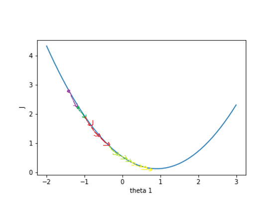
我们来直观地了解特征尺度归一化的梯度下降的过程。这里只展示单变量回归梯度下降过程。
In [134]:
X_show = X[:,0:2]
X_show = preprocess_data(X_show)

theta_0 = np.linspace(-2, 3, 50)
theta_1 = np.linspace(-2, 3, 50)
theta_0, theta_1 = np.meshgrid(theta_0,theta_1)
J = np.zeros_like(theta_0)

for i in range(50):
    for j in range(50):
        predict_Y = compute_predict_Y(X_show, np.array([[2.877],[theta_0[i,j]],[theta_1[i,j]]]))
        J[i,j] = compute_J(predict_Y, Y)

plt.contourf(theta_0, theta_1, J, 10, alpha = 0.6, cmap = plt.cm.coolwarm)
C = plt.contour(theta_0, theta_1, J, 10, colors = 'black')

# 画出损失函数J的历史位置
history_num = len(theta_history)
theta_0_history = np.zeros(history_num)
theta_1_history = np.zeros(history_num)
for i in range(history_num):
    theta_0_history[i],theta_1_history[i] = theta_history[i][2,0],theta_history[i][1,0]
plt.scatter(theta_0_history, theta_1_history, c="r")
Out[134]:
<matplotlib.collections.PathCollection at 0x7fcdc891b550>

可以看到,的值不断地往最低点移动。与没有进行特征尺度归一化的图相比,归一化后,每个维度的变化幅度大致相同,这有助于
的值快速下降到最低点。
正规方程
对于求函数极小值问题,可以使用求导数的方法,令函数的导数为0,然后求解方程,得到解析解。正规方程正是使用这种方法求的损失函数的极小值,而线性回归的损失函数
是一个凸函数,所以极小值就是最小值。
正规方程的求解过程就不详细推导了,正规方程的公式是:
如果,那么
是奇异矩阵,即
不可逆。
不可逆的原因可能是:
- 特征之间冗余,比如特征向量中两个特征是线性相关的。
- 特征太多,删去一些特征再进行运算。
正规方程的缺点之一就是不可逆的情况,可以通过正则化的方式解决。另一个缺点是,如果样本的个数太多,特征数量太多(
),正规方程的运算会很慢(求逆矩阵的运算复杂)。
任务10: 下面来实现正规方程。 提示:Numpy 求逆矩阵的函数是np.linalg.inv。
In [135]:
def normal_equation(X, Y):
    """正规方程求线性回归方程的参数 theta
    参数:
        X: 训练集数据特征,shape: (m, n+1)
        Y: 训练集数据标签,shape: (m, 1)
    返回:
        theta: 线性回归方程的参数
    """

    ### START CODE HERE ###

    theta = np.dot(np.dot(np.linalg.inv(np.dot(X.T,X)),X.T),Y)

    ### END CODE HERE ###

    return theta
In [136]:
theta = normal_equation(X, Y)

print("theta = ", theta)
theta =  [[2.861875  ]
 [0.70215497]
 [0.0417454 ]]
恭喜,你已经帮助项目负责人计算出了一个线性模型。
任务11: 假设明天的最高温度是°C,人口
百万,使用通过正规方程计算得到的
预测明天的城市的峰值用电量(单位:GW)吧!
注意,要进行同样的特征尺度归一化处理。
In [138]:
def predict(theta,x):

    ### START CODE HERE ###
    # 零均值单位方差归一化
    X = data[:,0:2].reshape((-1, 2))
    Y = data[:,2].reshape((-1, 1))

    mu = np.mean(X,axis=0)
    sigma = np.std(X,axis=0)

    x = (X-mu)/sigma

    # 在x前面加一列
    x = preprocess_data(x)
    #预测
    prediction = compute_predict_Y(x,theta)
    ### END CODE HERE ###

    return prediction

x = np.array([[40,3.3]])
print('预计明天的峰值用电量为:%.2f GW'%(predict(theta,x)[0]))
预计明天的峰值用电量为:3.72 GW
以上都是线性模型,当我们数据的特征与
的关系没有明显的线性关系,而且又找不到合适的映射函数时,可以尝试多项式回归。 下面导入另一组最高气温与用电量数据,我们用线性模型试一试看看效果发现并不太好。
In [140]:
data1 = np.loadtxt('/content/drive/MyDrive/data1.txt')
X = data1[:,0].reshape(-1,1)
Y = data1[:,1].reshape(-1,1)

plt.scatter(X,Y)
X = np.hstack((np.ones((X.shape[0],1)),X))
theta = normal_equation(X,Y)
plt.plot(np.sort(X[:,1]),np.dot(X,theta)[np.argsort(X[:,1])],'r')
Out[140]:
[<matplotlib.lines.Line2D at 0x7fcdc8d46390>]

多项式回归
多项式回归的最大优点就是可以通过增加的高次项对实测点进行逼近,直至满意为止。事实上,多项式回归可以处理相当一类非线性问题,它在回归分析中占有重要的地位,因为任一函数都可以分段用多项式来逼近。因此,在通常的实际问题中,不论依变量与其他自变量的关系如何,我们总可以用多项式回归来进行分析。假设数据的特征只有一个
,多项式的最高次数为
,那么多项式回归方程为:
若令
,那么
这就变为多变量线性回归了。
任务12:现在训练一个多项式模型,,直接用上面的正规方程得到模型。
所以输入数据
应该变成这样
In [141]:
data1 = np.loadtxt('/content/drive/MyDrive/data1.txt')
X = data1[:,0].reshape(-1,1)
Y = data1[:,1].reshape(-1,1)

### START CODE HERE ###

# 对X 前面加1, 后面加平方,变为 m x 3 的矩阵
m = X.shape[0]   # m 是数据X的行数
X_square = np.power(X,2)
X = np.hstack((X,X_square))
X = preprocess_data(X)

# 用正规方程求解theta
theta = normal_equation(X, Y)

### END CODE HERE ###
plt.scatter(X[:,1],Y)
plt.plot(np.sort(X[:,1]),np.dot(X,theta)[np.argsort(X[:,1])],'r')
Out[141]:
[<matplotlib.lines.Line2D at 0x7fcdc8fef5d0>]

所有任务到这里就结束了,下面是对上面的数据进行任意多项式拟合的结果,你可以通过多次改变的值来调整多项式的阶数来看看模型的效果(但不设的太大,
)。可以看到,越复杂的模型,虽然拟合数据效果很好,但是其泛化能力就会很差,所以模型应该要尽量简单。
In [142]:
from sklearn.linear_model import LinearRegression
from sklearn.preprocessing import PolynomialFeatures
from sklearn.pipeline import Pipeline
from sklearn.preprocessing import StandardScaler

def PolynomialRegression(degree):
    return Pipeline([
        ("poly",PolynomialFeatures(degree=degree)),
        ("std_scaler",StandardScaler()),
        ("lin_reg",LinearRegression())
    ])
X = data1[:,0].reshape(-1,1)
Y = data1[:,1].reshape(-1,1)
K = 193  #试试193(K<=193)

poly_reg = PolynomialRegression(degree=K)
poly_reg.fit(X,Y.squeeze())
y_predict = poly_reg.predict(X)
plt.scatter(X,Y)
plt.plot(np.sort(X[:,0]),y_predict[np.argsort(X[:,0])],color='r')
Out[142]:
[<matplotlib.lines.Line2D at 0x7fcdb593ef10>]


0 条评论